Using AI to Predict if a Paper will be in a Top-Tier Journal

I have been doing some work in recent months with Dr. Sophia Wang at Stanford applying deep learning/AI techniques to make predictions using notes written by doctors in electronic medical records (EMR). While the mathematics behind the methods can be very sophisticated, tools like Tensorflow and Keras make it possible for people without formal training to apply them more broadly. I wanted to share some of what I’ve learned to help out those who want to start with similar work but are having trouble with getting started.

For this tutorial (all code available on Github), we’ll write a simple algorithm to predict if a paper, based solely on its abstract and title, is one published in one of the ophthalmology field’s top 15 journals (as gauged by h-index from 2014-2018). It will be trained and tested on a dataset comprising every English-language ophthalmology-related article with an abstract in Pubmed (the free search engine operated by NIH covering practically all life sciences-related papers) published from 2010 to 2019. It will also incorporate some features I’ve used on multiple projects but which seem to be lacking in good tutorials online such as using multiple input models with tf.keras and tf.data, using the same embedding layer on multiple input sequences, and using padded batches with tf.data to incorporate sequence data. This piece also assumes you know the basics of Python 3 (and Numpy) and have installed Tensorflow 2 (with GPU support), BeautifulSoup, lxml, and Tensorflow Datasets.

Ingesting Data from Pubmed

Update: 21 Jul 2020 – It’s recently come to my attention that Pubmed turned on a new interface starting May 18 where the ability to download XML records in bulk for a query has been disabled. As a result the instructions below will no longer work to pull the data necessary for the analysis. I will need to do some research on how to use the E-utilities API to get the same data and will update once I’ve figured that out. The model code (provided you have the titles and abstracts and journal names extracted in text files) will still work, however.

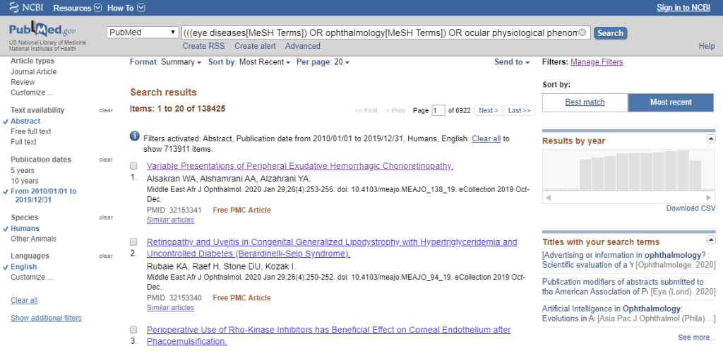
To train an algorithm like this one, we need a lot of data. Thankfully, Pubmed makes it easy to build a fairly complete dataset of life sciences-related language content. Using the National Library of Medicine’s MeSH Browser, which maintains a “knowledge tree” showing how different life sciences subjects are related, I found four MeSH terms which covered the Ophthalmology literature: “Eye Diseases“, “Ophthalmology“, “Ocular Physiological Phenomena“, and “Ophthalmologic Surgical Procedures“. These can be entered into the Pubmed advanced search interface and the search filters on the left can be used narrow down to the relevant criteria (English language, Human species, published from Jan 2010 to Dec 2019, have Abstract text, and a Journal Article or a Review paper):

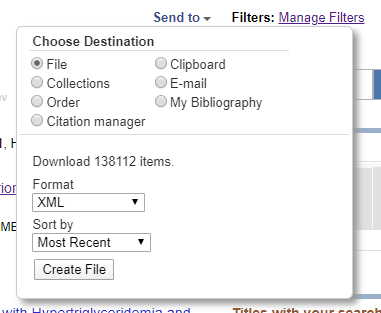
We can download the resulting 138,425 abstracts (and associated metadata) as a giant XML file using the “Send To” in the upper-right (see screenshot below). The resulting file is ~1.9 GB (so give it some time)

A 1.9 GB XML file is unwieldy and not in an ideal state for use in a model, so we should first pre-process the data to create smaller text files that will only have the information we need to train and test the model. The Python script below reads each line of the XML file, one-by-one, and each time it sees the beginning of a new entry, it will parse the previous entry using BeautifulSoup (and the lxml parser that it relies on) and extract the abstract, title, and journal name as well as build up a list of words (vocabulary) for the model.

The XML format that Pubmed uses is relatively basic (article metadata is wrapped in <PubmedArticle> tags, titles are wrapped in <ArticleTitle> tags, abbreviated journal names are in <MedlineTA> tags, etc.). However, the abstracts are not always stored in the exact same way (sometimes in <Abstract> tags, sometimes in <OtherAbstract> tags, and sometimes divided between multiple <AbstractText> tags), so much of the code is designed to handle those different cases:

After parsing the XML, every word in the corpus that shows up at least 25 times (smallestfreq) is stored in a vocabulary list (which will be used later to convert words into numbers that a machine learning algorithm can consume), and the stored abstracts, titles, and journal names are shuffled before being written (one per line) to different text files.

Looking at the resulting files, its clear that the journals Google Scholar identified as a top 15 journal in ophthalmology are some of the more prolific journals in the dataset (making up 8 of the 10 journals with the most entries). Of special note, ~21% of all articles in the dataset were published in one of the top 15 journals:

Journal	Short Name	Top 15 Journal?	Articles as % of Dataset
Investigative Ophthalmology & Visual Science	Invest Ophthalmol Vis Sci	Yes	3.63%
PLoS ONE	PLoS One	No	2.84%
Ophthalmology	Ophthalmology	Yes	1.99%
American Journal of Ophthalmology	Am J Ophthalmol	Yes	1.99%
British Journal of Ophthalmology	Br J Ophthalmol	Yes	1.95%
Cornea	Cornea	Yes	1.90%
Retina	Retina	Yes	1.75%
Journal of Cataract & Refractive Surgery	J Cataract Refract Surg	Yes	1.64%
Graefe’s Archive for Clinical and Experimental Ophthalmology	Graefes Arch Clin Exp Ophthalmol	No	1.59%
Acta Ophthalmologica	Acta Ophthalmol	Yes	1.40%
All Top 15 Journals		~	21.3%

Building a Model Using Tensorflow and Keras

Translating even a simple deep learning idea into code can be a nightmare with all the matrix calculus that needs to done. Luckily, the AI community has developed tools like Tensorflow and Keras to make this much easier (doubly so now that Tensorflow has chosen to adopt Keras as its primary API in tf.keras). It’s now possible for programmers without formal training (let alone knowledge of what matrix calculus is or how it works) to apply deep learning methods to a wide array of problems. While the quality of documentation is not always great, the abundance of online courses and tutorials (I personally recommend DeepLearning.ai’s Coursera specialization) bring these methods within reach for a self-learner willing to “get their hands dirty.”

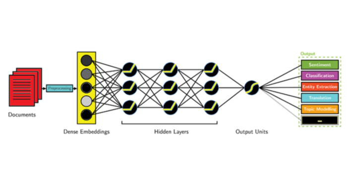
As a result, while we could focus on all the mathematical details of how the model architecture we’ll be using works, the reality is its unnecessary. What we need to focus on are what the main components of the model are and what they do:

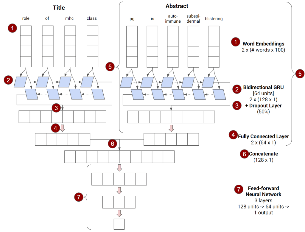
1. The model converts the words in the title into vectors of numbers called Word Embeddings using the Keras Embedding layer. This provides the numerical input that a mathematical model can understand.
2. The sequence of word embeddings representing the abstract is then fed to a bidirectional recurrent neural network based on Gated Recurrent Units (enabled by using a combination of the Keras Bidirectional layer wrapper and the Keras GRU layer). This is a deep learning architecture that is known to be good at understanding sequences of things, something which is valuable in language tasks (where you need to differentiate between “the dog sat on the chair” and “the chair sat on the dog” even though they both use the same words).
3. The Bidirectional GRU layer outputs a single vector of numbers (actually two which are concatenated but that is done behind the scenes) which is then fed through a Dropout layer to help reduce overfitting (where an algorithm learns to “memorize” the data it sees instead of a relationship).
4. The result of step 3 is then fed through a single layer feedforward neural network (using the Keras Dense layer) which results in another vector which can be thought of as “the algorithm’s understanding of the title”
5. Repeat steps #1-4 (using the same embedding layer from #1) with the words in the abstract
6. Combine the outputs for the abstract (step 4) and title (step 5) by literally sticking the two vectors together to make one larger vector — and then run this combination through a 2-layer feedforward neural network (which will “combine” the “understanding” the algorithm has developed of both the abstract and the title) with an intervening Dropout layer (to guard against overfitting).
7. The final layer should output a single number using a sigmoid activation because the model is trying to learn to predict a binary outcome (is this paper in a top-tier journal [1] or not [0])

The above description skips a lot of the mathematical detail (i.e. how does a GRU work, how does Dropout prevent overfitting, what mathematically happens in a feedforward neural network) that other tutorials and papers cover at much greater length. It also skims over some key implementation details (what size word embedding, what sort of activation functions should we use in the feedforward neural network, what sort of random variable initialization, what amount of Dropout to implement).

But with a high level framework like tf.keras, those details become configuration variables where you either accept the suggested defaults (as we’ve done with random variable initialization and use of biases) or experiment with values / follow convention to find something that works well (as we’ve done with embedding dimension, dropout amount, and activation function). This is illustrated by how relatively simple the code to outline the model is (just 22 lines if you leave out the comments and extra whitespace):

Building a Data Pipeline Using tf.data

Now that we have a model, how do we feed the data previously parsed from Pubmed into it? To handle some of the complexities AI researchers regularly run into with handling data, Tensorflow released tf.data, a framework for building data pipelines to handle datasets that are too large to fit in memory and/or where there is significant pre-processing work that needs to happen.

We start by creating two functions

1. encode_journal which takes a journal name as an input and returns a 1 if its a top ophthalmology journal and a 0 if it isn’t (by doing a simple comparison with the right list of journal names)
2. encode_text which takes as inputs the title and the abstract for a given journal article and converts them into a list of numbers which the algorithm can handle. It does this by using the TokenTextEncoder function that is provided by the Tensorflow Datasets library which takes as an input the vocabulary list which we created when we initially parsed the Pubmed XML

These methods will be used in our data pipeline to convert the inputs into something usable by the model (as an aside: this is why you see the .numpy() in encode_text — its used to convert the tensor objects that tf.data will pass to them into something that can be used by the model)

Because of the way that Tensorflow operates, encode_text and encode_journal need to be wrapped in tf.py_function calls (which let you run “normal” Python code on Tensorflow graphs) which is where encode_text_map_fn and encode_journal_map_fn (see code snippet below) come in.

Finally, to round out the data pipeline, we:

1. Use tf.data.TextLineDataset to ingest the text files where the parsed titles, abstracts, and journal names reside
2. Use the tf.data.Dataset.zip method to combine the title and abstract datasets into a single input dataset (input_dataset).
3. Use input_dataset‘s map method to apply encode_text_map_fn so that the model will consume the inputs as lists of numbers
4. Take the journal name dataset (journal_dataset) and apply its map method to apply encode_journal_map_fn so that the model will consume the inputs as 1’s or 0’s depending on if the journal is one of the top 15
5. Use the tf.data.Dataset.zip method to combine the input (input_dataset) with the output (journal_dataset) in a single dataset that our model can use

To help the model generalize, its a good practice to split the data into four groups to avoid biasing the algorithm training or evaluation on data it has already seen (i.e. why a good teacher makes the tests related to but not identical to the homework), mainly:

1. The training set is the data our algorithm will learn from (and, as a result, should be the largest of the four).
2. (I haven’t seen a consistent name for this, but I create) a stoptrain set to check on the training process after each epoch (a complete run through of the training set) so as to stop training if the resulting model starts to overfit the training set.
3. The validation set is the data we’ll use to compare how different model architectures and configurations are doing once they’ve completed training.
4. The hold-out set or test set is what we’ll use to gauge how our final algorithm performs. It is called a hold-out set because its not to be used until the very end so as to make it a truly fair benchmark.

tf.data makes this step very simple (using skip — to skip input entries — and take which, as its name suggests, takes a given number of entries). Lastly, tf.data also provides batching methods like padded_batch to normalize the length of the inputs (since the different abstracts and titles will have different lengths, we will truncating or pad each title to be 72 words and 200 words long, respectively) between the batches of 100 articles that the algorithm will train on successively:

Training and Testing the Model

Now that we have both a model and a data pipeline, training and evaluation is actually relatively straightforward and involves specifying which metrics to track as well as specifics on how the training should take place:

• Because the goal is to gauge how good the model is, I’ve asked the model to report on four metrics (Sensitivity/Recall [what fraction of journal articles from the top 15 did you correctly get], Precision [what fraction of the journal articles that you predicted would be in the top 15 were actually correct], Accuracy [how often did the model get the right answer], and AUROC [a measure of how good your model trades off between sensitivity and precision]) as the algorithm trains
• The training will use the Adam optimizer (a popular, efficient training approach) applied to a binary cross-entropy loss function (which makes sense as the algorithm is making a yes/no binary prediction).
• The model is also set to stop training once the stoptrain set shows signs of overfitting (using tf.keras.callbacks.EarlyStopping in callbacks)
• The training set (train_dataset), maximum number of epochs (complete iterations through the training set), and the stoptrain set (stoptrain_dataset) are passed to model.fit to start the training
• After training, the model can be evaluated on the validation set (validation_dataset) using model.evaluate:

After several iterations on model architecture and parameters to find a good working model, the model can finally be evaluated on the holdout set (test_dataset) to see how it would perform:

Results

Your results will vary based on the exact shuffle of the data, which initial random variables your algorithm started training with, and a host of other factors, but when I ran it, training usually completed in 2-3 epochs, with performance resembling the data table below:

Statistic	Value
Accuracy	87.2%
Sensitivity/Recall	64.9%
Precision	72.7%
AUROC	91.3%

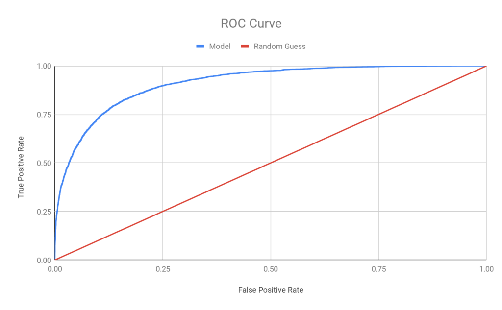
A different way of assessing the model is by showing its ROC (Receiver Operating Characteristic) curve, the basis for the AUROC (area under the ROC curve) number and a visual representation of the tradeoff the model can make between True Positives (on the y-axis) and False Positives (on the x-axis) as compared with a purely random guess (blue vs red). At >91% AUROC (max: 100%, min: 50%), the model outperforms many common risk scores, let alone a random guess:

Interestingly, despite the model’s strong performance (both AUROC and the point estimates on sensitivity, precision, and accuracy), it wasn’t immediately apparent to me, or a small sample of human scientists who I polled, what the algorithm was looking for when I shared a set of very high scoring and very low scoring abstracts and titles. This is one of the quirks and downsides of many AI approaches — their “black box” nature — and one in which followup analysis may reveal more.

Special thanks to Sophia Wang and Anthony Phan for reviewing abstracts and reading an early version of this!

Link to GitHub page with all code